Read Kafka like a Database
Working with Kafka data on your own terms, using a local index.
A search stack usually follows Kafka into a service. But the message you are looking for is already in the topic — and what format it is in, which fields are worth indexing, the data says for itself. Pick a topic and the index builds itself.
Why this exists
I have used Kafka in services for a long time — tracing user actions, propagating events for event sourcing, moving work between pipeline steps. And every time, the same ecosystem went up around it. ELK, so that someone could search the messages when operations or an incident called for it. A sink connector, to forward data into some persistent store. ksqlDB, or Flink, to count and watch the stream. More infrastructure, more software.
Then one day a thought crossed my mind.
Kafka processes a message stream sequentially, through a consumer. So if I do not know the partition and offset of the needle, I have to look for it from the beginning. But if I do know them — can I reach the message directly, the way I would in any other database?
ELK was not necessary on that service. I only needed to find trace events, and they were already sitting in the topic. All I needed to know was where.
The usual Kafka architecture
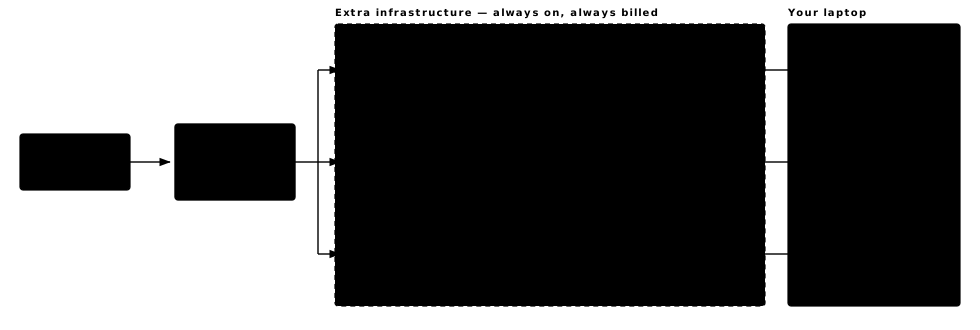
To search messages you wire Kafka Connect (or Logstash) into Elasticsearch, a sink connector into a database, and ksqlDB or Flink for counting. Each one is a service that has to be up, upgraded and paid for, and each one is reached through a different client.
Building out a data pipeline is good work for a data engineer — interesting, and good for a career. Running cost is a separate matter. The more systems there are to manage, the more it takes to build them and to keep them running.
Inside a company that cost is somebody else's budget, so it is easy not to feel. On a service you are funding yourself, you feel all of it.
So it is worth asking plainly: does the service need the pipeline, or does it just need to find a message?
What makes a local index possible
A Kafka topic is append-only, ordered within a partition, and addressable by offset. An index over it is
therefore a pure function of (topic, partition, offset range) — it can be built incrementally,
and resumed from wherever it stopped, without coordinating with anything else.
None of this needs new technology. SQLite, DuckDB, RocksDB and plenty of others can hold an index on local disk; which one to reach for gets a section of its own further down. And an index sitting beside a consumer is already familiar here — Kafka Streams keeps its state in RocksDB, ksqlDB with it. The only thing that changes is which machine the consumer runs on.
A lighter architecture: Kafka and a local index
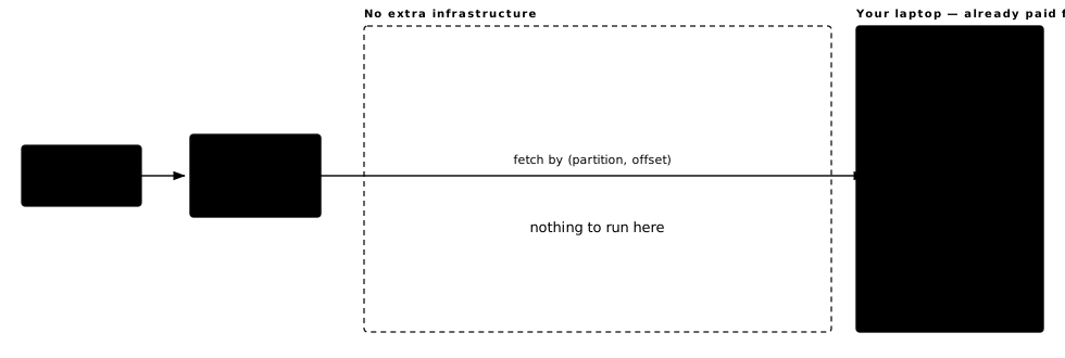
Fetch by explicit partition and offset, build the index locally, search it locally — the local-first version of the same idea. No consumer group is joined and no offsets are committed, so the cluster does not notice.
For each message it reads the key, the headers and the value, decodes them in whatever format the topic
turned out to be in, and walks the result. Every scalar it finds becomes a term — the path it sat under,
and the value there — and a field can be split into words as well, when that is how you would go looking
for it. Each term is written down with the (partition, offset) it came from.
That is the whole of it: a sorted map from term to positions, and one record per message holding what a result row needs to show. Nothing else is kept, which is why the body still has to be fetched when you open one.
Scanning versus looking up
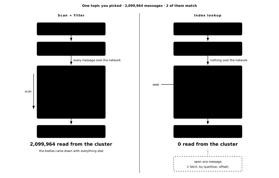
Without an index there is only one way to find a message: scan the topic and filter client-side. The work is proportional to the topic, not to the answer — two matches in two million messages still costs two million reads across the network, and refining the query costs them again.
An index inverts that. Terms are stored in sorted order, so a prefix seek lands directly on the block that
matches and reads nothing on either side of it. Each entry carries a (partition, offset) and
enough to render a row, so the whole result list is built without asking the cluster for anything — zero
reads, however many times the query is refined. Indexing pays for one read up front; everything
after it is proportional to the number of hits.
The fields that were indexed are in the index, so building the result list asks the cluster for
nothing. Only opening one of those rows needs the original message, and that fetch names exactly
one by (partition, offset). If no consumer group is joined there are no offsets to
commit, so no rebalance is triggered and nobody else's position moves.
Search needs an index first
The search above leaves one thing out. A search runs against an index, and until a topic is indexed there is nothing in it to find. Building that index means reading the topic through once.
That read is not an extra one, though. A scan would have pulled every message across anyway and then thrown the work away; indexing moves the same bytes and keeps what it found. What it adds is the work per message — decode it, derive terms, write them down — and that is the whole of the difference. It is also paid once, where the scan pays its share again on every query.
Given the data, indexing configures itself
Most of what a pipeline makes you declare up front is already in the data. Sample the messages and the wire format falls out of the bytes, the fields worth indexing out of what actually appears in them. Formats that rely on a schema registry say what they are too — the message carries its schema id, so an address for the registry is the whole of the setup. Past those few choices, the indexing runs itself.
How long indexing takes
So the time goes on that per-message work, not on the reading. Keep it small and a million messages is a wait you sit through rather than schedule. Figures from the implementation are in the appendix.
The whole topic is read once
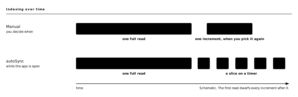
The last indexed offset is recorded per partition, so nothing is ever read twice. Leave a topic on manual
and it catches up in one step the next time you pick it or press sync; turn on autoSync and it
keeps up in slices while the app is open. Either way the full read happens once, and an interrupted one
resumes where it stopped rather than starting over.
My desktop and yours are too powerful, and too expensive, to use only for a web browser and a chat window.
What it costs on disk
A fair question by now: can one machine hold an index over what a Kafka cluster has been accumulating?
Managed well, an index does not swell far beyond the messages it describes. The cost is per field and per message, so it can be judged before a byte is read. Figures in the appendix.
So the question is not how large the cluster is, but how much of it you keep. There is no reason to take all of it. The topics you search, the fields you actually use, as far back as you need to look — that much fits on one machine.
Not indexing everything
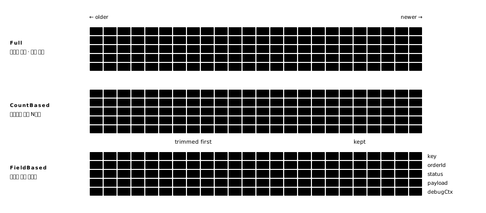
The three are set in different places. Topics are decided when you pick them; count and fields are a cleanup policy, and can be tightened after the fact.
| Strategy | What it trims | Setting |
|---|---|---|
| Index only the topics you actually search | whole topics | — |
| Keep the newest N per partition | messages | CountBased |
| Keep only the fields you search | fields | FieldBased |
If index size starts to matter, not every field has to be in it. A Kafka payload tends to carry all sorts, and the fields you would never search — the encoded ones, the long prose — can be left out. Cost falls per field, so the index comes down in proportion to what you drop. Cutting one JSON topic to the fields actually searched took about a fifth off.
When the disk fills anyway
The strategies above are choices made up front. Alongside them there has to be a ceiling that holds whatever those choices were: a size budget over the index as a whole, checked on a timer, reclaiming space without being asked once it is passed. Garbage collection, in effect — nobody has to remember to run it.
What gets reclaimed is governed by per-topic policies, and each one is a different answer to the same question: what is the cheapest thing to stop knowing? These are the ones that exist today.
| Policy | What it gives up |
|---|---|
| CountBased | older messages stop being searchable |
| FieldBased | those fields stop being searchable |
| DropIndex | the topic goes back to unindexed |
| … | the list is open — sampling one message in N is the obvious next one, and anything that trades a little detail for a lot of room belongs here |
A discarded index is not lost data. The messages are still in Kafka, and picking the topic again builds it back. That is the difference between reclaiming space here and dropping a table in a database you own — and it is why the cleanup can be left to run unattended.
Where to put the index
By now the index has shown what it demands: long sustained writes while a topic is taken on, seeks to a sorted prefix on every search, and slices thrown away whenever a policy trims.
| SQLite B-tree, FTS5 | DuckDB columnar | RocksDB LSM tree | |
|---|---|---|---|
| Good at | ranked full-text, substrings via trigrams | SQL and aggregation over large data | sustained writes, cheap bulk deletion |
| Costs you | index size grows fast; trimmed space needs reclaiming | indexes cover = and IN; a prefix lookup is still a scan, and trimming rewrites data |
matching is yours to build, n-grams included |
| Pick it when | the data fits comfortably | the answer is an aggregate | the data keeps growing |
I went with RocksDB for the implementation all of this is drawn from; it gets its name at the end. The first two hand over much of the indexing work already done, which is a real convenience to give up. But ksqlDB reaches for RocksDB for a reason, and it is the same one here: an LSM tree matches the way Kafka data accumulates, and holds its performance as the pile keeps growing.
What that costs is the key design, the tokenizing and the rest of the matching, all written by hand — and it cuts both ways. The query planning is yours as well — how a lookup runs is something you decide and tune for the data at hand, rather than something a library settles behind an interface you cannot reach.
Keys kept in sorted order buy two moves: jump to an exact value, or to where a given prefix begins.
Nothing past that comes free. Matching a word
inside a sentence means tokenizing before the write. Matching part of a word means an n-gram index — a
second index, with a size of its own. So it comes down to a choice: carry that size to support
%oo%, or leave it out and stay small.
And how those keys are designed is what the implementation turns on.
Where a local index stops
A local index is not always the answer. Some things only a pipeline can do. Here the two are set side by side, and the limits are gathered toward the bottom.
| Pipeline | Local index | |
|---|---|---|
| Before the first search | install and wire Connect, Elasticsearch and Kibana, then write the mapping | install an app, then one read of the topic |
| Operating | always on; versions, shards, disk | none |
| Fixed cost | instances, every month | none — hardware you own |
| Where the data goes | replicated out of the cluster | stays on your disk |
| Load on the cluster | continuous replication of everything | one read to index, then only what you open |
| Matching | analyzers, wildcards, partial words | values, prefixes and whole words |
| Scale ceiling | add nodes, scale sideways | whatever one machine holds — growable, still one machine |
| Sharing with a team | everyone sees the same view | no — each disk is its own |
| Retention | keep it forever | Kafka retention plus local trimming |
| Ongoing use | lands in a warehouse, a database, some persistent layer | only when a person opens it |
If the index will not fit on one machine, if a team has to share one view, or if the data must outlive Kafka's retention, the pipeline is the right answer. The largest of the four is the last row: if the data has to end up somewhere permanent — a warehouse, a database, whatever reads from it downstream — an index that runs only when someone opens it cannot stand in for that. A local index only works where none of those four applies.
In short
- Given the data, indexing configures itself. The format and the useful fields fall out of the data, so past a few choices there is no mapping to write, no schema to register and no connector to configure.
- The index is a pure function of what it has read, because a topic is addressable by offset. So the full read happens once — the read a scan would have done anyway — and after that only increments, resumed wherever they stopped.
- The index does not swell far beyond the messages it describes, and comes down with every field and every message you leave out of it.
- A search runs entirely in the local index, so it costs the cluster nothing. Only opening a message goes back to Kafka, by explicit partition and offset.
- Where it does not cover you: when the index will not fit on one machine, when a team has to share one view, when the data must outlive Kafka's retention, and when something has to serve as a persistent store.
Conclusion
Kafka is a good data store — it scales horizontally, it stays up, it answers quickly. A great many services run on it for good reasons.
A data pipeline usually follows, because that is how Kafka tends to get used.
But the data is already in Kafka. Give a topic an index it builds for itself, and it reads the way a database does — straight to the message rather than walking to it.
If Kafka is going into a service, the version with a local index is worth sketching too.
The architecture above is implemented in Kaflow Search, a local-first desktop application you install on your own machine.
macOS 11+ · Windows 10+ · free, no account needed Not signed yet — the first launch needs the usual override. There is a demo build if you have no cluster to point it at.
Appendix: numbers from Kaflow Search
These came off Kaflow Search on an M4 with 32 GB, on RocksDB with its default compression. A different machine or store lands somewhere else, so take the absolute figures as a reference.
Indexing rate
| Topic | Fields | Rate | 100K msgs | 1M msgs |
|---|---|---|---|---|
| chat-messages | 19 | about 10,000 / sec | about 10 sec | about 100 sec |
Fields counted as below — about 19 values per message, from 15 declared ones once the list-valued fields are expanded. The laptop was the limit here, not the network: a faster machine does more, a remote cluster less.
Disk
Four topics, a million messages each, every field indexed. Raw message is the key, the value and the headers as plain JSON, before anyone compresses anything; stored locally is what RocksDB ends up holding, messages and the index over them together. Bytes per message read straight across as megabytes per million.
Indexing every field runs 1.1 to 1.2 times the raw data — raw meaning the data itself, not what the Kafka cluster keeps on disk. Tokenizing, or building n-grams, makes search finer and the index larger in proportion. zstd can bring it under that, by how much depends on the data.
| Topic | Fields | Raw / msg | Stored / msg | With zstd | 100K msgs | 1M msgs |
|---|---|---|---|---|---|---|
| inventory-events | 21 | 515 B | 586 B1.14× | 418 B0.81× | 64 MB | 586 MB |
| notification-events | 22 | 593 B | 673 B1.14× | 516 B0.87× | 71 MB | 673 MB |
| payments-events | 26 | 636 B | 768 B1.21× | 483 B0.76× | 79 MB | 768 MB |
| crawled-market-signals | 31 | 840 B | 927 B1.10× | 656 B0.78× | 90 MB | 927 MB |
The last two columns also say the shape holds: ten times the messages came out at 0.92 to 1.03 times the size per message, so a small sample predicts a large topic. In principle, 100 GB of local disk covers well over a hundred million messages. Holding that much locally is not what this is for, though.
The last two columns are at the default compression, snappy. zstd can trim more but can also slow writes; the two trade off.